A Decade of Premier League Football

The English Premier League is BACK!

Before we get over-excited, let's have a look at the past. Here is a shiny app to visualise some stats from last ten seasons. It is my first attempt at developing data-driven sports stories with R, Shiny and Shiny Dashboard. Those stories ain't new, but I had always wanted to visualise the data instead of just reading them from articles.

It includes the last-minute title decider in 2011-2012 season (I am a red devil. That. Still. Hurts.) ...

... as well as the survival race.

Enjoy. Code is on GitHub.

Got some interesting football stories in mind? Free feel to give me a shout and see if we can create some more data viz.

What's Next?

I am actually more interested in predicting match outcomes and fantasy football. In the coming months, I am going to include more predictive modelling stuff.

On the other hand, I am also working on some new ggplot2 geom (e.g. geom_football, geom_basketball) for sports data visualisation. Hopefully, I can give you an update on this soon.

TTTAR2: My First Shiny App with Bootstrap - #RUGSMAPS

Thing To Try After useR! part 2 (TTTAR2)

Originally, this post was supposed to be a sequel to TTTAR1 about h2o machine learning. Since TTTAR1 I have been carrying out more h2o tests both locally and on the cloud with the very kind support of Nick Elprin from Domino. The more I find out about h2o and Domino, the more I get addicted. So my original plan was to write a new post about combining the best of h2o and Domino - building a scalable data analytic platform on the cloud with R as the main interface.

Well something happened unexpectedly so here is a change of plan – I am going to talk about Shiny web application and data visualisation again. I will get back to h2o machine learning and Domino later. In the meantime, check out Nick’s recent blog post about Domino which is directly relevant to what I am planning to blog next.

Beautiful Shiny Apps at useR!

I know how to use Shiny and Bootstrap. Yet, before useR!, I had never felt the need to combine them. Shiny already has a clean and tidy layout by default – so why bother changing it? But then I changed my mind completely after useR!. There were quite a few beautiful Shiny apps with custom CSS on display. For example, during the second poster session, I saw this amazing Shiny app created by Christian Gonzalez and Robert Youmans.

When I had the chance to play with the app on Christian’s laptop, that sleek and professional interface just completely blew my mind. It was at this moment I realised that I was wrong and it’s time to up my game.

Revolution Analytics Data Visualisation Contest

Just like how I learned about maps in R last year, I needed to find something interesting and dive into it. After useR!, I read about this contest from Joseph’s post. It seemed like a good data visualisation exercise with a small and tabulated dataset. It was also a good opportunity to combine Shiny and rMaps (something that I hadn’t managed to do when I last worked on rCrimemap many months ago).

The Making of R User Groups Maps (RUGSMAPS)

Many thanks to the detailed Shiny examples from RStudio and Chris Beeley’s book as well as the huge rCharts/rMaps contributions by Ramnath Vaidyanathan and Kenton Russell on GitHub and Stackoverflow, I didn't need to spend much time on coding as many useful code snippets are just one Google search away.

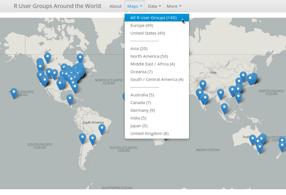
I did, however, spend a lot more time on the layout design and user interface. Font size, colours, white spaces, choice of base map etc you name it. I also tried quite a few Bootstrap themes and finally settled with Spacelab. I am not the best person to describe the final design with correct art terminology. I just feel that this combination of blue, grey and white gives a clean layout (yet not too flashy). The RUGSMAPS app is currently hosted on ShinyApps (once again, thanks RStudio!!!)

Don't agree with my colour choices? No worries, fork the repository and modify the boostrap.css in the www folder. More information can be found on the "About" page of the app so I am not going to repeat it here. Please try it out and tell me what you think about it.

What's Next?

As the RUGSMAPS app is my final submission to the contest, I am going to lock down the version so the app becomes a reference point version 1. Further improvements will be made independently (let’s just call it RUGSMAPS v2 for now). The idea is to collect more local information from the RUGs and display it accordingly on the maps. For example, in additional to the group name and city location, I can include more information such as usual meetup location, key sponsors, website, photos etc.

I have seen a cool example from Alex Bresler that shows images in the markers’ pop-up window. I am certain that we can display more information than just the group name and city location. BTW, Alex and his colleagues at Aragorn Technologies are doing some very cool interactive sports data visualisation with R for huge events (e.g. NBA, US Open) – do check them out!!!

Together We Can Make It Better! 

If you have some local information about the RUGs and are interested in improving the RUGSMAPS for the community, please drop me an email (jofai.chow@gmail.com), comment on this post or create issues on the repository. We can make this a central info hub of all RUGs! Let’s do it!!!

Acknowledgement 

First of all, I would like to thank Revolution Analytics (David and Joseph) for the award! I would also like to emphasise that the RUGSMAPS app did not just come out of my head from nowhere. It is the direct result of many cool ideas I learned and borrowed from the R community over the last year or so. To all my R friends I met on Twitter / GitHub / useR!, if you're reading this, you know I am talking about you. So thank you very much everyone!

The Rise of R in Hydroinformatics

(View from the Empire State Building Observatory - it was at this moment I realised that I should begin my career as Batman)

Just a bit off the topic, I attended the Hydroinformatics conference in New York last week and I witnessed the rise of R in this field. Although MATLAB still seems the most common programming language (ever wonder why my twitter handle sounds a bit too odd?), there were more talks about using R for Hydroinformatics this time (compared to none in the same conference two years ago). People were presenting their R packages and discussing how they use R for interfacing as well as teaching. RStudio IDE was on the big screen several times!

Yet, still no sight of Shiny but I think I can change that!!!

rCharts Parcoords x Simpsons x Blocks

Interactive Parallel Coordinates with Multiple Colours

For my research project, I need a tool to visualise results from multi-objective optimisations. Below is one of my early attempts using base R and parcoord in the MASS package, I have no problem using them for publication. However, these charts are all static. For a practical decision support tool (something I am working on), I need the charts to be interactive so that users can adjust the range/thresholds in each parameter and narrow down the things to display in real time.

Many thanks to Ken (timelyportfolio) who kindly pointed me to his code examples. Based on that, I developed a prototype version of the interactive parallel coordinates plot with multiple colours (as shown above). OK, the values in the chart are totally unrelated to my research - I just used the 'Theoph' dataset in R for testing purposes. Yet, this is a much needed exercise to see if I can use rCharts parallel coordinates for my research. The answer, of course, is YES. It also works with my customised colour palette too (using Bart Simpson this time)!

Click here to view the he Interactive Version

Here is the R code for the above chart:

Showing your rCharts on bl.ocks.org

In the process of making this plot, I also discovered how to display rCharts (d3, html or practically any code) on Mike Bostock's site "bl.ocks.org". If you haven't seen his site, do check this out. It is one of the coolest things on earth.

I wanted to have a gallery like that too ... but I didn't know how. I used to think that Ramnath and Ken must have bought Mike a beer so that they can have their stuff hosted on bl.ocks.org (see bl.ocks.org/ramnathv and bl.ocks.org/timelyportfolio). I was very wrong, everyone with a GitHub account can do it. All you need are your imagination (and some gists). The site automatically pulls your gists and displays them as beautiful blocks gallery.

In order to display your cool rCharts on bl.ocks.org, you can either:

1. publish the rCharts to gist using the '$publish' function (e.g. r1$publish('name.of.gist', host = 'gist')  where r1 is the rCharts object)
2. save the rCharts as a stand-alone HTML (e.g. r1$save('index.html', cdn = TRUE)) and then include it in a gist.

For optimal display, I would recommend setting your rCharts size to 960 x 500 (same as the display size on bl.ocks.org). You can also include a 'README.md' file and a 'thumbnail.png' to provide more information. I think the best resolution for the thumbnail is 230 x 120 (about the same aspect ratio as full display). You will need to manually push the png file (see this post for more details).

So here are the parallel coodinates plot as shown on bl.ocks.org ...

... and my gallery at bl.ocks.org/woobe

Latest on Colour Palette Generator

First, let me point you to Russell Dinnage's blog post. It is easily one of the finest R blog posts I've read so far. All these colours and graphs. Wow! It's yet another #RCanDoThat moment for me (so good it needs a hashtag).

So many thanks to his effort and cool ideas, we continue to add more functions to the rPlotter package. It is also a great opportunity for us to better understand the pull/merge GitHub mechanism.

Credits

Again, I would like to thank Ken for his help (not only this time but many times before this on visualisation stuff) as well as Ramnath, Mike and Russell.

Towards (Yet) Another R Colour Palette Generator. Step One: Quentin Tarantino.

Why?

I love colours, I love using colours even more. Unfortunately, I have to admit that I don't understand colours well enough to use them properly. It is the same frustration that I had about one year ago when I first realised that I couldn't plot anything better than the defaults in Excel and Matlab! It was for that very reason, I decided to find a solution and eventually learned R. Still learning it today.

What's wrong with my previous attempts to use colours? Let's look at CrimeMap. The colour choices, when I first created the heatmaps, were entirely based on personal experience. In order to represent danger, I always think of yellow (warning) and red (something just got real). This combination eventually became the default settings.

"Does it mean the same thing when others look at it?"

This question has been bugging me since then. As a temporary solution for CrimeMap, I included controls for users to define their own colour scheme. Below are some examples of crime heatmaps that you can create with CrimeMap.

Personally, I really like this feature. I even marketed this as "highly flexible and customisable - colour it the way you like it!" ... I remember saying something like that during LondonR (and I will probably repeat this during useR later).

Then again, the more colours I can use, the more doubts I have with the default Yellow-Red colour scheme. What do others see in those colours? I need to improve on this! In reality, you have one chance, maybe just a few seconds, to tell your very important key messages and to get attention. You can't ask others to tweak the colours of your data visualisation until they get what it means.

Therefore, I know another learning-by-doing journey is required to better understand the use of colours. Only this time, I already have about a year of experience with R under my belt, I decided to capture all the references, thinking and code in one R package.

Existing Tools

Given my poor background in colours, a bit of research on what's available is needed. So far I have found the following. Please suggest other options if you think I should be made aware of (thanks!). I am sure this list will grow as I continue to explore more options.

Online Palette Generator with API

• http://www.colourlovers.com/ (with colourlovers R interface)
• http://www.pictaculous.com/ (the results are nice. Yet, the API has a 500kb image size limit)

Key R Packages

• RColorBrewer by Erich Neuwirth - been using this since very first days
• colorRamps by Tim Keitt - another package that I have been using for a long time
• colorspace by Ross Ihaka et al. - important package for HCL colours
• colortools by Gaston Sanchez - for HSV colours
• munsell by Charlotte Wickham - very useful for exploring and using Munsell colour systems

Funky R Packages and Posts:

• wesanderson by Karthik Ram - love this! Give this a go and if you haven't tried it yet.
• RSkittleBrewer by Alyssa Frazee - funky Skittle and M&M colour schemes
• Further points on crayon colors by Karl Broman - another interesting set of colours!

Other Languages:

• Color Thief by Lokesh Dhakar (JavaScript)

The Plan

"In order to learning something new, find an interesting problem and dive into it!" - This is roughly what Sebastian Thrun said during "Introduction to A.I.", the very first MOOC I participated. It has a really deep impact on me and it has been my motto since then. Fun is key. This project is no exception but I do intend to achieve a bit more this time. Algorithmically, the goal of this mini project can be represented as code below:

> is.fun("my.colours") & is.informative("my.colours")
> TRUE

Seriously speaking, based on the tools and packages mentioned above, I would like to develop a new R package that does the following five tasks. Effectively, these should translate into five key functions (plus a sixth one as a wrapper that goes through all steps in one go).

1. Extracting colours from images (local or online).
2. Selecting and (adjusting if needed) colours with web design and colour blindness in mind.
3. Arranging colours based on colour theory.
4. Evaluating the aesthetic of a palette systematically (quantifying beauty).
5. Sharing the palette with friends easily (think the publish( ) and load_gist( ) functions in Shiny, rCharts etc).

I decided to start experimenting with colourful movie posters, especially those from Quentin Tarantino. I love his movies but I also understand that those movies might be offensive to some. That is not my intention here as I just want to bring out the colours. If these examples somehow offend you, please accept my apologies in advance.

First function - rPlotter :: extract_colours( )

The first step is to extract colours from an image. This function is based on dsparks' k-means palettle gist. I modified it slightly to include the excellent EBImage package for easy image processing. For now, I am including this function with my rPlotter package (a package with functions that make plotting in R easier - still in early development).

Note that this is the very first step of the whole process. This function ONLY extracts colours and then returns the colours in simple alphabetical order (of the hex code). The following examples further illustrate why a simple extraction alone is not good enough.

Example One - R Logo

Let's start with the classic R logo.

So three-colour palette looks OK. The colours are less distinctive when we have five colours. For the seven-colour palette, I cannot tell the difference between colours (3) and (5). This example shows that additional processing is needed to rearrange and adjust the colours, especially when you're trying to create a many-colour palette for proper web design and publication.

Example Two - Kill Bill

What does Quentin_Tarantino see in Yellow and Red?

Actually the results are not too bad (at least I can tell the differences).

Example Three - Palette Tarantino

OK, how about a palette set based on some of his movies?

I know more work is needed but for now I am quite happy playing with this.

Example Four - Palette Simpsons

Don't ask why, ask why not ...

I am loving it!

Going Forward

So the above examples show my initial experiments with colours. It will be, to me, a very interesting and useful project in long-term. I look forward to making some sports related data viz when the package reaches a stable version.

The next function in development will be "select_colours()". This will be based on further study on colour theory and other factors like colour blindness. I hope to develop a function that automatically picks the best possible combination of original colours (or adjusts them slightly only if necessary). Once developed, a blog post will follow. Please feel free to fork rPlotter and suggest new functions.

useR! 2014

If you're going to useR! this year, please do come and say hi during the poster session. I will be presenting a poster on the crime maps projects. We can have a chat on CrimeMap, rCrimemap, this colour palette project or any interesting open-source projects.

Acknowledgement

I would like to thank Karthik Ram for developing and sharing the wesanderson package in the first place. I asked him if I could add some more colours to it and he came back with some suggestions. The conversation was followed by some more interesting tweets from Russell Dinnage and Noam Ross. Thank you all!

I would also like to thank Roland Kuhn for showing how to embed individual files of a gist. This is the first time I embed code here properly.

Tweets are the easiest way for me to discuss R these days. Any feedback or suggestion, Tweet to @matlabulous

Updates on Interactive rCrimemap, rBlocks ... and the Packt offer!

Testing rCrimemap as a Self-Contained Web Page

I've been learning more about rMaps and rCharts since the LondonR meeting. There are many amazing things you can do with rCharts but it does take time to learn all the tweaks. For example, I just discovered that the rMaps objects (like other rCharts ojects) can be saved as a self-contained webpage.

So here are the links to one of the maps I rendered with rCrimemap - visualising all the England, Wales and N. Ireland crimes in Jan 2014 (not sure why some of the crimes were recorded in Scotland - I'll need to further investigate this later). Eventually, I hope to build a new Shiny web app for rCrimemap that allows users to change the settings like the original CrimeMap.

Link 1 - rCrimemap (1900 x 1060)

Link 2 - rCrimemap (940 x 620)

Note: I would recommend NOT to try this on smartphones. I will need to figure out how the map can be trimmed and optimised for smartphones later.

Yet Another rBlocks Experiment

Playing with the EBImage package this time, I wrote this script to pixelate a picture and re-colour it with rBlocks (just for fun - not practical at all ...) (Gist - rBlocks_test_04_pixelation.R)

Celebrating Packt's 2000th Book

Finally, Packt is offering "Buy One Get One Free" on all ebooks to celebrate the 2000th title!!!

The #rBlocks Experiments

What's this ?

Where should I start? OK, the story goes like this ...

rBlocks: A port of #ipythonblocks to #rstats http://t.co/iMMRPCxQIN @simplystats @gvwilson @hadleywickham pic.twitter.com/6LQmN4LZWM
— Ramnath Vaidyanathan (@ramnath_vaidya) March 12, 2014

Colouring #rstats df with @ramnath_vaidya #rBlocks Iris revisited http://t.co/TFDDXGK7y2 nvr thought df can be funky? pic.twitter.com/ue2ajM0ZXQ
— Jo-fai Chow (@matlabulous) March 18, 2014

@matlabulous Cool application! I am trying to make this easier by trying to squeeze color and values into same structure.
— Ramnath Vaidyanathan (@ramnath_vaidya) March 18, 2014

@ramnath_vaidya thanks! With auto colours we can visualise the process of evolutionary optimisation or model ensembles quickly with #rBlocks
— Jo-fai Chow (@matlabulous) March 18, 2014

@matlabulous Feel free to suggest features on github.
— Ramnath Vaidyanathan (@ramnath_vaidya) March 18, 2014

@ramnath_vaidya done :) https://t.co/8HoCYSrWBr
— Jo-fai Chow (@matlabulous) March 18, 2014

@ramnath_vaidya another go at #rBlocks exploratory analysis on 'AirPassengers'. This time with #RSkittleBrewer! pic.twitter.com/kcZYYDmyVl
— Jo-fai Chow (@matlabulous) March 19, 2014

Conway's Game of Life animated using #rstats #rBlocks #animation @ramnath_vaidya @xieyihui http://t.co/VegpVUqSKn http://t.co/b1zMQzDrcN
— Jo-fai Chow (@matlabulous) March 19, 2014

@Jowanza did you read my mind? http://t.co/VegpVUqSKn http://t.co/b1zMQzDrcN
— Jo-fai Chow (@matlabulous) March 19, 2014

What's next? Let's go crazy with colours ... (to be continued)

Slidify my R journey from @matlabulous to rCrimemap

My LondonR Talk

Thanks to Mango Solutions (LondonR organiser), I was given the opportunity last night to talk about my mini project ‘CrimeMap’. Instead of going through all the technical details behind the scenes, I chose to talk the audience through my R journey from a noob to a heavy user. CrimeMap was used as a case study to show how ones can benefit from learning R (or, in some ways, trying to justify the time I spent staring at RStudio IDE last year). The feedback was really great and the talk effectively expanded my network in the data science community so I am really grateful for that! You can find my presentation here.

Before the main event, there was an excellent R-Python workshop by Chris Musselle. The other two interesting presentations were "Dynamic Report Generation" by Kate Hanley and "Customer Clustering for Retail Marketing" by Jon Sedar. Their presentations will soon be made available here.

CrimeMap - A Wonderful Learning Experience

When I first started learning R for real, the goal was very simple - "let's plot something pretty with ggplot2". Well, a lot has changed since then. The more I learned, the more I discovered. It is really hard to summarise the 'R' awesomeness in a few slides due to its diversity. One thing I am absolutely certain is that I made the right move about a year ago to shift from MATLAB to R. Yet, I am keeping my twitter account name @matlabulous just to remind myself that ones should always keep an open mind for new and evolving technology (... and should avoid getting a tattoo of your potential ex-gf/bf's name. On that note, no, I don't have a tattoo.) For more information about the CrimeMap, please see my previous posts here, here and here.

Using Slidify for Professional Presentation

The talk was also the first time I presented something totally unrelated to water engineering. I thought, for a change, let’s try something different. Then I remembered looking at the Slidify slides from Jeff Leek’s Data Analysis course back in Jan-March last year. I thought that would fit perfectly for LondonR because the whole presentation would be coded completely in R. It would be a good reason to learn Slidify too. So I went through the Slidify examples, put some slides together, tweaked the CSS a little bit and then published it to GitHub – a streamline Slidify workflow well thought and designed by Ramnath Vaidyanathan. To me, the results are amazing! So amazing that I am confident to leave PowerPoint and use Slidify for professional presentations in the future.

rMaps + CrimeMap = rCrimemap

Two weeks before the presentation, I wrote an email to Ramnath as I wanted to thank him for Slidify. I told him how I enjoyed using Slidify for the LondonR slides. Out of the blue, Ramnath told me that he had seen my CrimeMap already and he kindly pointed me to this blog post about using Leaflet heat map in rMaps. I thought, OMG, why now? Then I thought, yeah, why not? So I created a new package called ‘rCrimemap’ based on Ramnath’s example and the codes from the CrimeMap project – just in time for the LondonR meeting. At first, I wanted to called the package something different but eventually I chose rCrimemap so it aligns well with Ramnath’s rCharts and rMaps.

Using ‘rCrimemap’

rCrimemap is still raw and experimental. It depends on some new packages such as dplyr, dev version of rCharts and rMaps etc. I have only developed and tested it recently on Linux. Please give it a try if you have a chance. All feedback and suggestions are welcome. Codes are here.

To install it, you will need the RStudio IDE version 0.98.501 or newer and the following packages ...

require(devtools)
install.packages(c("base64enc", "ggmap", "rjson", "dplyr"))
install_github('ramnathv/rCharts@dev')
install_github('ramnathv/rMaps')

After that, install rCrimemap package via ... 

install_github('woobe/rCrimemap')

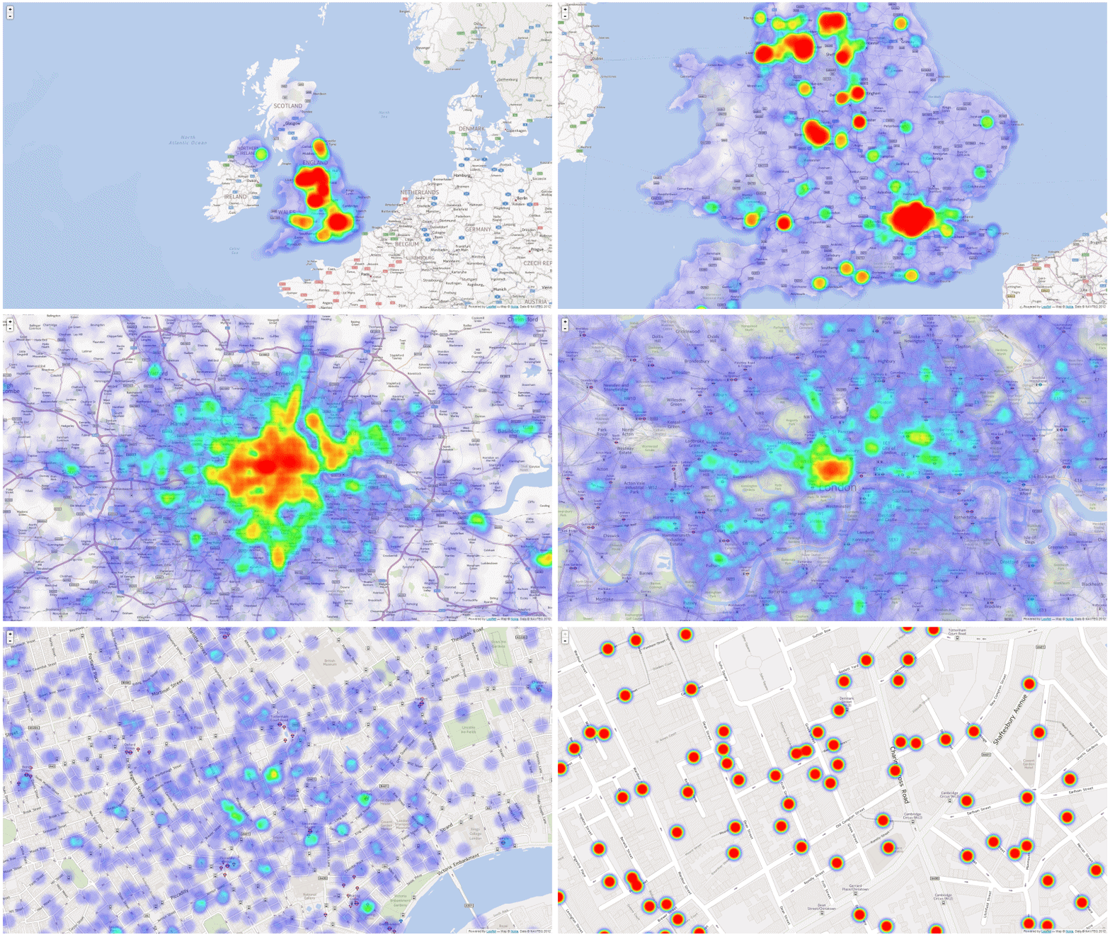
rCrimemap is basically a big wrapper function. In fact, there is only one function 'rcmap( )' in the package at the moment. (OK, it is obviously an overkill ... but I really wanted to try developing a package.) The function is very similar to the first one I did for CrimeMap prior to the Shiny development. In terms of graphical functionality, it is not as flexible as the CrimeMap yet (for example, CrimeMap can do all these colours and facet). However, it is much more powerful than CrimeMap in the sense that users can move around, zoom in and out like using a real digital map. The colour of the heat map also changes when you zoom in/out. This gives users a much better visibility of where the local crime hot spots are when they zoom in. OK, enough said, let’s go through some example usage …

The arguments of the function 'rcmap( )' are:

1. location: point of interest within England, Wales and Northern Ireland
2. period: a month between Dec 2010 and Jan 2014 (in the format of yyyy-mm)
3. type: category of crime (e.g. "All", "Anti-social behaviour")
4. map_size: the resolution of the map in pixel (e.g. Full HD = c(1920, 1080))
5. provider: the base map provider (e.g. "Nokia.normalDay", "MapQuestOpen.OSM")
6. zoom: zoom level of the map (e.g. I recommend starting with 10 to show all the crimes)

Example 1: “Ball Brothers EC3R 7PP” (LondonR venue since March 2013) during the London riot (Aug 2011). The map can be viewed within RStudio IDE or be exported to a browser. The animation was created outside R (Oh ... what if rCrimemap + animation package? ... I will leave that for later.)

rcmap("Ball Brothers EC3R 7PP", "2011-08", "All", c(1000,1000),"Nokia.normalDay")

Example 2: Manchester in Jan 2014 - using "MapQuestOpen.OSM" as base map instead.

rcmap("Manchester", "2014-01", "All", c(1000,1000), "MapQuestOpen.OSM")

Credits

There you go, enjoy :)

Introducing CrimeMap - A Web App Powered by ShinyApps!

A few months ago I did a mini project using open crime data and R to create crime visualisations. At that time, I was already thinking about a web app using Shiny but I couldn't justify the time to develop the app and then set up a server etc. Not until two weeks ago when I received an invitation to join the alpha testing of ShinyApps.

ShinyApps - A Wonderful Discovery

I went through the ShinyApps' getting started guide. Everything looks pretty straight forward. So I decided to go ahead and moved my codes from the crime visualisation project to a new ShinyApps project. The progress was unexpectedly smooth. Given that I had no web application development experience prior to this mini exercise, I consider this a quick success! All credit goes to the RStudio team for providing these tools and hosting services (especially Tareef Kawaf who kindly answered all my questions). I would summarise the whole process in the following few steps:

1. Sign up for a ShingApps alpha testing account here (you will need a Google account).
2. Install packages shiny and shinyapps (click on the links for installation help).
3. Sign in to my.shinyapps.io, give your ShinyApps account a name ("blenditbayes" in my case) and get your application token/secret.
4. Go through the tutorials, create the ui.R and server.R scripts for your app.
5. Test the app locally using runApp().
6. Once you're happy with the app, apply your token/secret and deploy your app using deployApp().

That's it! I can focus my effort solely on developing the app. The rest has been taken care of and simplified by the deployApp() and other ShinyApps functions.
 

CrimeMap in Action

So here is my first ever web app "CrimeMap" powered by ShinyApps! I will go through the usage briefly in the following sections. I hope you can give it a try and give me some feedback (e.g. what features are missing?) so I can continue to improve it. Your comments will be valuable to the ShinyApps development team too.

URL: http://blenditbayes.shinyapps.io/crimemap/

Basic Usage

First, enter a location of your choice (e.g. London) within England, Wales and Northern Ireland. Select the first month of crime data collection and then the length of the analysis period. After that, click on the "Update" button. My experience is that the graphs should come up within a minute if the length of analysis is less than or equal to 6 months. Depending on the location and the length of analysis, the process might take longer (say a couple minutes). The outputs (at the time of writing) are displayed in three tabs: Data, Crime Map and Trends. The Data tab shows the original crime data records downloaded from the data.police.uk (I may add a feature like "download as CSV in future). The crime map is a density plot of the crime data. Finally, the trends tab shows bar charts of crime records over time in different crime categories. Right click on the map and you can save the image in its original size (1280 x 1280).

Customise the Maps

Continue to scroll down the menu on the left, you will find more settings for the map. Change the facet settings to create map facets according to crime type, categories and month. You can select different Google map format (roadmap, satellite, hybrid or terrain). There are also options to download the Google map image in high resolution (it takes a bit longer), in black & white and at various zoom levels. When you click the "Update" button to refresh the maps, it may take a while to show the new graphs if you have lots of facets.

Fine-tuning the Density Plots

The Density Plot Settings allow user to modify the "behind the scenes" ggplot2 codes. You can modify the layer transparency (alpha range), the number of bins, the width and the colour of the boundary lines as well as the colours of the gradient. My hope is to develop a user-friendly interface that allows users to quickly create maps with their own favourite themes. Surely, ggplot2 is much more powerful than that and has a lot more settings available. What other settings would you like to see here? Please let me know.

Exploring the Trends

Why am I including the trends visualisation? It just happened that I read this article around the same time I received the ShinyApps invitation. As I had already coded something for crime data visualisation, I thought it would be interesting to look at the data myself. So here is a handy tool for you to explore and to visualise the data with a few clicks. I will leave you with your own conclusions.

Feedback Please

As I mentioned above, I am new to web app development and this is my first ever experiment. Please have a go, create a few maps and let me know what can be done better. Thanks in advance!! All the codes are available here.

Visualising Crime Hotspots in England and Wales using {ggmap}

Two weeks ago, I was looking for ways to make pretty maps for my own research project. A quick search led me to some very informative blog posts by Kim Gilbert, David Smith and Max Marchi. Eventually, I Google'd the excellent crime weather map example by David Kahle and decided to stick with the gg-style approach.

Thanks to David Kahle and Hadley Wickham who ramped up that example and subsequently developed the {ggmap} package, making maps in R can be really intuitive and fun!

I wrote a wrapper function that takes a location within England and Wales, downloads crime data around that location over a certain period of time and creates crime weather plots. This blog post discusses the data used, methodology and the wrapper function with some worked examples. The codes are available here.

(Nov-2013 Update: I have updated the codes and created a web app using Shiny and ShinyApps. For more information, please read this new blog post.)

Data

The street-level crime data is one of the 9,000 datasets available from data.gov.uk. The data can be downloaded systematically via the Police API. The latest version of the API no longer requires authentication.

The following URL can be used to obtain crime records at street-level within a one-mile radius of a single point. The parameters required are latitude, longitude and month. The downloaded data is in JSON format which can be converted into R's data format using the {RJSONIO} package.

Example URL: http://data.police.uk/api/crimes-street/all-crime?lat=52.629729&lng=-1.131592&date=2012-04

Methodology

The methodology can be summarised in the following six steps:

1. Obtain latitude and longitude of a user-defined location using ggmap::geocode.
2. Download crime data via the Police API as discussed above.
3. Convert JSON into a list and then a data frame.
4. Download a base map from Google using ggmap::get_googlemap.
5. Covert the base map into a ggplot object using ggmap::ggmap.
6. Add multiple layers on top of the base map using the data frame like a normal ggplot.

For more details, check out the functions in the codes:

• "get.data" and "list2df" for steps 1, 2 and 3
• "visualise.data" for steps 4, 5 and 6

Wrapper and Worked Examples

The wrapper function looks like this ...

crimeplot.wrapper <- function(
  point.of.interest = "London Eye",  ## user-defined location
  period = c("2013-01","2013-02"),  ## period of time in YYYY-MM
  type.map = "roadmap",  ## roadmap, terrain, satellite or hybrid
  type.facet = NA,  ## options: NA, month, category or type
  type.print = NA,  ## options: NA, panel or window
  output.plot = TRUE,  ## print it to a png file?
  output.filename = "temp.png",  ## provide a filename
  output.size = c(700,700)) ## width and height setting                              

... given the location, time period and a few more graphical settings, the wrapper can produce a crime weather map. The following worked examples illustrate the usage.

Example 1 - All crimes around London Eye from Jan-2013 to Apr-2013

Comments:
Here we can see a huge crime hotspt in the Soho district of London - an area full of bars, restaurants, theatres and nightclubs (did I mention Chinatown?)

Codes:
## Define the period
ex1.period <- format(seq(as.Date("2013-01-01"),length=4,by="months"),"%Y-%m")

## Use the wrapper
ex1.plot <- crimeplot.wrapper(point.of.interest = "London Eye",
                              period = ex1.period,
                              type.map = "roadmap",
                              output.filename = "ex1.png",
                              output.size = c(700,700))

Example 2 - Typical crimes and traffic incidents around London Eye from Jan-2013 to Apr-2013

(Note: click on the image to see original image in higher resolution)

Comments:
Now we seperate the data from British Transport Police (BTP) and all other forces (Force) using the facet function in {ggplot}. We can see a traffic black spot on the other side of River Thames.

Codes:

## Define the period
ex2.period <- format(seq(as.Date("2013-01-01"),length=4,by="months"),"%Y-%m")
 
## Use the wrapper
ex2.plot <- crimeplot.wrapper(point.of.interest = "London Eye",
                              period = ex2.period,
                              type.map = "roadmap",
                              type.facet = "type",
                              output.filename = "ex2.png",
                              output.size = c(1400,700))

Example 3 - Monthly crimes in Manchester for the year 2012 on a satellite map

(Note: click on the image to see original image in higher resolution)

Comments:
Using the facet function on "month", we can look at the changes in patterns over time. Looks like there is not much seasonality in Manchester as the crime hotspots remain hot over the year.

Codes:

## Define the period
ex3.period <- format(seq(as.Date("2012-01-01"),length=12,by="months"),"%Y-%m")

## Use the wrapper
ex3.plot <- crimeplot.wrapper(point.of.interest = "Manchester",
                              period = ex3.period,
                              type.map = "satellite",
                              type.facet = "month",
                              output.filename = "ex3.png",
                              output.size = c(1400,1400))

Example 4 - Crimes by categories in Liverpool from Jan-2013 to Apr-2013 on a hybrid map

(Note: click on the image to see original image in higher resolution)

Comments:
Now we separate different categories of crimes. It is interesting to see that only a small part of the city is affected by shoplifting and other theft while burglary, arson and vehicle crimes are very common problems in Liverpool.

Codes:

## Define the period
ex4.period <- format(seq(as.Date("2013-01-01"),length=4,by="months"),"%Y-%m")
 
## Use the wrapper
ex4.plot <- crimeplot.wrapper(point.of.interest = "Liverpool",
                              period = ex4.period,
                              type.map = "hybrid",
                              type.facet = "category",
                              output.filename = "ex4.png",
                              output.size = c(1400,1400))

Further Work

Further work is needed to ...
1. optimise the codes for "list2df" transformation (At the moment it is quite slow. I tried lapply but it didn't give me back the desired data frame format but I know there must be a solution.)
2. better automate the graphical settings for output resolution, font size etc.
3. make it interactive using {Shiny}

(Nov-2013 Update: I have improved (1) using plyr::ldply and done (2 & 3). See this.)

Acknowledgement

I would like to thank Yanchang Zhao for his excellent book titled "R and Data Mining: Examples and Case Studies" which encouraged me to shift from MATLAB to R. All embedded codes were Created by Pretty R at inside-R.org.

Key References

1. David Kahle's original crime map.

2. Police API documentation.